This is particularly useful when working with lists copied and pasted from withing software (like WordPress or Drupal). Perhaps you are making a list of blogs you have written or you want to check the order of a menu: often when you copy this data you get spare bits of html such as button names or tooltips pasting over, and it’s a pain to remove them manually.
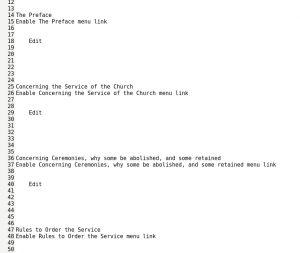
Today, I had a list of 400 Durpal pages in a menu that I wanted to check the order of, comparing them to lists which I know were correct. The initial copy and paste was a real mess:
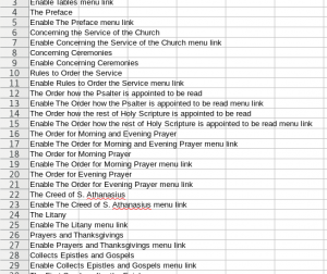
First, I removed some extra lines and things using the methods mentioned here and here. Then I pasted the content into a LibreOffice Calc sheet.
As you can see, every other line is a button title to enable a menu link – those are not needed! So lets remove them.
Table of Contents
Add descending numbers
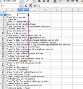
First, you will need an empty row at the top of the sheet.
Then put a number 1 next to the first item, in the next column over: drag or click to auto-fill the column with ascending numbers.
Add a mod
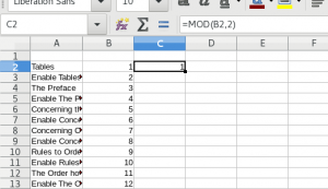
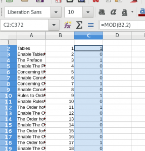
Next, click the adjacent cell in the next column over and (assuming you want to remove every other row) put in:
=MOD(top number in sequence, 2)
so in my example that was:
=MOD(B2, 2)
If you want to remove every 3rd row you could but 3, every 4th row, 4 and so on.
Again, drag or click down to autofill.
You should see 1, 0, 1, 0 if you are selecting every other row, or 1, 2, 3, 1, 2, 3 if you are selecting every 3rd row.
Filter
Finally, select the whole column, and go
Data > AutoFilter
Click yes if it asks “Do you want the first line to be used as column header?”
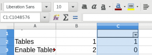
You will now see a little drop-down in the first cell of that column:
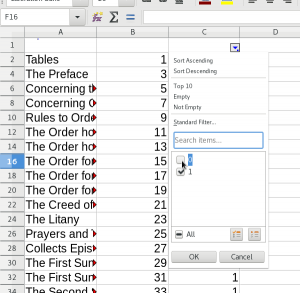
Click the drop-down and uncheck the line number you want to delete: in my case this is zero, in the image above “Tables” (which I want to keep) has a 1 in row C but “Enable Tables…” (which I want to lose) has a zero. So I un-check zero.
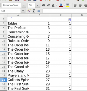
Now all the ones are visible but the zeros are gone!
If you made a mistake, you can change the settings on the auto-filter.
Enjoy!
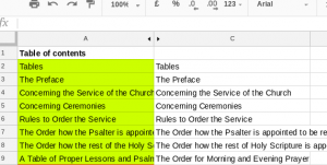
I can now check if my items are in order – and I can already spot an error, so I am glad to checked!
Thanks, that just saved me a lot of time
I know this has some age on it – But I found it useful today. That being said as slight update for those that may not know it… MOD’s format has been changed slightly to:
=MOD(B2; 2)
From
=MOD(B2, 2)
They changed “,” to “;”. This is as of 4.1.14.
Thanks for the update thats great, I’ll try and update this sometime in the blog. Sorry for delay replying I had a baby x